Getting Started with CMS 2010 Open Data
- "I have installed the CERN Virtual Machine: now what?"
- "Do I have to use a virtual machine?"
- "OK! Where can I get the CMS data?"
- "Nice! But how do I analyse these data?"
- Option A: Analysing the primary dataset
- Option B: Analysing reduced datasets
- Performing your analysis on the PATtuples
"I have installed the CERN Virtual Machine: now what?"
To analyse CMS data collected in 2010, you need version 4.2.8 of CMSSW, supported only on Scientific Linux 5. If you are unfamiliar with Linux, take a look at this short introduction to Linux or try this interactive command-line bootcamp. Once you have installed the CMS-specific CERN Virtual Machine, you need to open a terminal. In the "CMS-OpenData-1.1.2" VM, always use the "CMS shell" terminal available from the "CMS Shell" icon on the desktop (only if using the VM version "CMS-OpenData-1.0.0-rc7", open a terminal with the X terminal emulator from an icon bottom-left of the VM screen). Execute the following command in the terminal if you haven't done so before; it ensures that you have this version of CMSSW running:
$ cmsrel CMSSW_4_2_8
Then, make sure that you are always in the CMSSW_4_2_8/src/ directory and the CMS analysis environment is properly setup by entering the following commands in the terminal (you must do so every time you boot the VM before you can proceed):
$ cd CMSSW_4_2_8/src/
$ cmsenv
"Do I have to use a virtual machine?"
Not necessarily. You can also try to analyse CMS data in a Docker container instead of in a virtual machine. If you are interested in that, instructions are here.
"OK! Where can I get the CMS data?"
It is best if we start off with a quick introduction to ROOT. ROOT is the framework used by several particle-physics experiments to work with the collected data. Although analysis is not itself performed within the ROOT GUI, it is instructive to understand how these files are structured and what data and collections they contain.
The primary data provided by CMS on the CERN Open Data Portal is in a format called "Analysis Object Data" or AOD for short. These AOD files are prepared by piecing raw data collected by various sub-detectors of CMS and contain all the information that is needed for analysis. The files cannot be opened and understood as simple data tables but require ROOT in order to be read.
So, let's see what an AOD file looks like and take ROOT for a spin!
Make sure that you are in the CMSSW_4_2_8/src/ folder (and in the "CMS Shell" terminal, if using the "CMS-OpenData-1.1.2" VM), and you have executed the cmsenv command in your terminal to launch the CMS analysis environment.
You can now open a CMS AOD file in ROOT. Let us open one of the files from the CERN Open Data Portal by entering the following command:
$ root root://eospublic.cern.ch//eos/opendata/cms/Run2010B/Mu/AOD/Apr21ReReco-v1/0000/00459D48-EB70-E011-AF09-90E6BA19A252.root
You will see the ROOT logo appear on screen. You can now open the ROOT GUI by entering:
TBrowser t
Excellent! You have successfully opened a CMS AOD file in ROOT. If this was the first time you've done so, pat yourself on the back. Now, to see what is inside this file, let us take a closer look at some collections of physics objects.
On the left window of ROOT (see the screenshot below), double-click on the file name (root://eospublic.cern.ch//eos/opendata/...). You should see a list of entries under Events, each corresponding to a collection of reconstructed data. We are interested in the collections containing information about reconstructed physics objects.
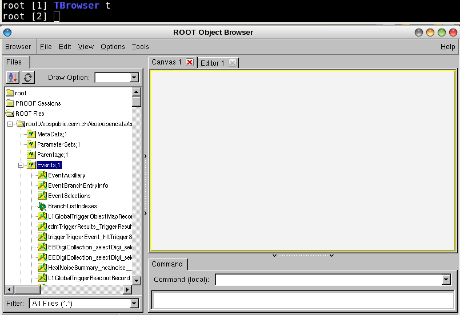
Let us take a peek, for example, at the electrons, which are found in recoGsfElectrons_gsfElectrons__RECO, as shown on the list of physics objects. Look in there by double-clicking on that line and then double-clicking on recoGsfElectrons_gsfElectrons__RECO.obj. Here, you can have a look at various properties of this collection, such as the plot for the transverse momentum of the electrons: recoGsfElectrons_gsfElectrons__RECO.obj.pt_.
You can exit the ROOT browser through the GUI by clicking on Browser on the menu and then clicking on Quit Root or by entering .q in the terminal.
"Nice! But how do I analyse these data?"
In AOD files, reconstructed physics objects are included without checking their "quality". For example, the reconstructed objects in the electron collection that you opened in ROOT were not actually verified to be electrons. In order to analyse only the "good quality" data, you must apply some selection criteria.
With these criteria, you are in effect reducing the dataset, either in terms of the number of collisions events it contains or in terms of the information carried by each event. Following this, you run your analysis code on the reduced dataset.
Depending on the nature of your analysis you can run your analysis code directly on the AOD files themselves, if needed, performing the selections along the way. However, this can be resource-intensive and is done only for very specific usecases.
NOTE: To analyse the full event content, the analysis job needs access to the "condition data", such as the jet-energy corrections. To see how the connection to the condition database is established, you can check the Guide to the CMS condition database. For simpler analyses, where we use only physics objects needing no further data for corrections, you do not need to connect to the condition database. This is the case for the example for analysing the primary datasets below.
Your final analysis is done using a software module called an "analyzer". If you have followed the validation step for the virtual machine setup, you have already produced and run a simple analyzer. You can specify your initial selection criteria within the analyzer to perform your analysis directly on the AOD files, or further elaborate the selections and other operations needed for analysing the reduced dataset. To learn more about configuring analyzers, follow these instructions in the CMSSW WorkBook. Make sure, though, that you replace the release version (CMSSW_nnn) with the release that you are using, i.e. one that is compatible with the CMS open data.
You can also pass the selection criteria through the configuration file. This file activates existing tools within CMSSW in order to perform the desired selections. If you have followed the validation step for the virtual machine setup, you have already seen a configuration file, which is used to give the parameters to the cmsRun executable. You can see how this is done in our analysis example.
We will now take you through these steps through a couple of specially prepared example analyses.
Option A: Analysing the primary dataset
As mentioned above, you do not typically perform an analysis directly on the AOD files. However, there may be cases when you can do so. Therefore, we have provided an example analysis to take you through the steps that you may need on the occassions that you want to analyse the AOD files directly. You can find the files and instructions in this CMS analysis example.
Option B: Analysing reduced datasets
We start by applying selection cuts via the configuration file and reduce the AOD files into a format known as PATtuple. You can find more information about this data format (which gets its name from the CMS Physics Analysis Toolkit, or PAT) on the CMSSW PAT WorkBook.
Important: Be aware that the instructions in the WorkBook are in use in CMS currently and have been updated for more recent CMSSW releases. With the 2010 data, you should always use the releases in the series of CMSSW_4_2 and not higher. Also note that more recent code does not work with older releases, so whenever you see git cms-addpkg... in the instruction, it is likely that the code package this command adds does not work with the release you need. However, the material under the pages gives you a good introduction to PAT.
Code as well as instructions for producing PATtuples from the CMS open data can be found in this GitHub repo. However, since it took a dedicated computing cluster nine days (!!!) to run this step and reduce the several TB of AOD files to a few GB of PATtuples, we have provided you with the PATtuples in that GitHub repo, saving you quite a lot of time! So you can jump to the next step, below ("Performing your analysis…"). Although you do not need to run this step, it is worth looking at the configuration file:
You can see that the line removeAllPATObjectsBut(process, ['Muons','Electrons']) removes all "PATObjects" but muon and electrons, which will be needed in the final analysis step of this example.
Note also how only the validated runs are selected on lines:
import FWCore.ParameterSet.Config as cms
import PhysicsTools.PythonAnalysis.LumiList as LumiList
myLumis = LumiList.LumiList(filename='Cert_136033-149442_7TeV_Apr21ReReco_Collisions10_JSON_v2.txt').getCMSSWString().split(',')
process.source.lumisToProcess = cms.untracked.VLuminosityBlockRange()
process.source.lumisToProcess.extend(myLumis)
This selection must always be applied to any analysis on CMS open data, and to do so you must have the validation file downloaded to your local area.
When using the "CMS-OpenData-1.1.2" VM, it is recommended reading the condition data as instructed in the Guide to the CMS condition database. Set the symbolic links to the condition database for 2010 data
ln -sf /cvmfs/cms-opendata-conddb.cern.ch/FT_R_42_V10A FT_R_42_V10A
ln -sf /cvmfs/cms-opendata-conddb.cern.ch/FT_R_42_V10A.db FT_R_42_V10A.db
Then replace the Global Tag definition on lines 45–46 in the file PAT_data_repo.py with
#globaltag
process.GlobalTag.connect = cms.string('sqlite_file:/cvmfs/cms-opendata-conddb.cern.ch/FT_R_42_V10A.db')
process.GlobalTag.globaltag = 'FT_R_42_V10A::All'
Performing your analysis on the PATtuples
Now, as the intermediate PATtuple files have been produced for you, you can go directly to the next step, as described in this second GitHub repo and follow the instructions on that page.
Note that even though these are derived datasets, running the analysis code over the full data can take several hours. So if you want just give it a try, you can limit the number events or read only part of the files. Bear in mind that running on a low number of files will not give you a meaningful plot.
Your analysis job is defined in OutreachExercise2010/DecaysToLeptons/run/run.py. The analysis code is in the files located in the OutreachExercise2010/DecaysToLeptons/python directory.
This example uses IPython, which gets configured and starts the job with the following command:
ipython run.py
That's it! Follow the rest of the instructions on the README and you have performed an analysis using data from CMS. Hope you enjoyed this exercise. Feel free to play around with the rest of the data and write your own analyzers and analysis code. To exit IPython, enter exit().

